Quasi-Cyclic LDPC: A Primer
Table of Contents
This is an ongoing blog post about LDPC codes, along with a Python implementation that’ll eventually be tangled as the blog post progresses. It is meant to be approachable, and glosses over details that are not useful from an implementation point of view to ensure that we do not get sidetracked.
1. Background
Stable high speed digital data transmission has great demand in the modern world. One major concern is controlling error in these transmissions. In his foundational paper A Mathematical Theory of Communication, Shannon presents the “Noisy channel coding theorem”, in which he proves that for any given channel with some amount of noise, it is possible to send error-free digital data (with suitable encoding) through it up to a certain rate called the Shannon limit. The problem we attempt to solve is understanding and implementing codes that are able to function close to this limit (capacity approaching codes). Chief among these are low density parity check (LDPC) codes, which are the subject of this article.
1.1. The Setup: BPSK over AWGN
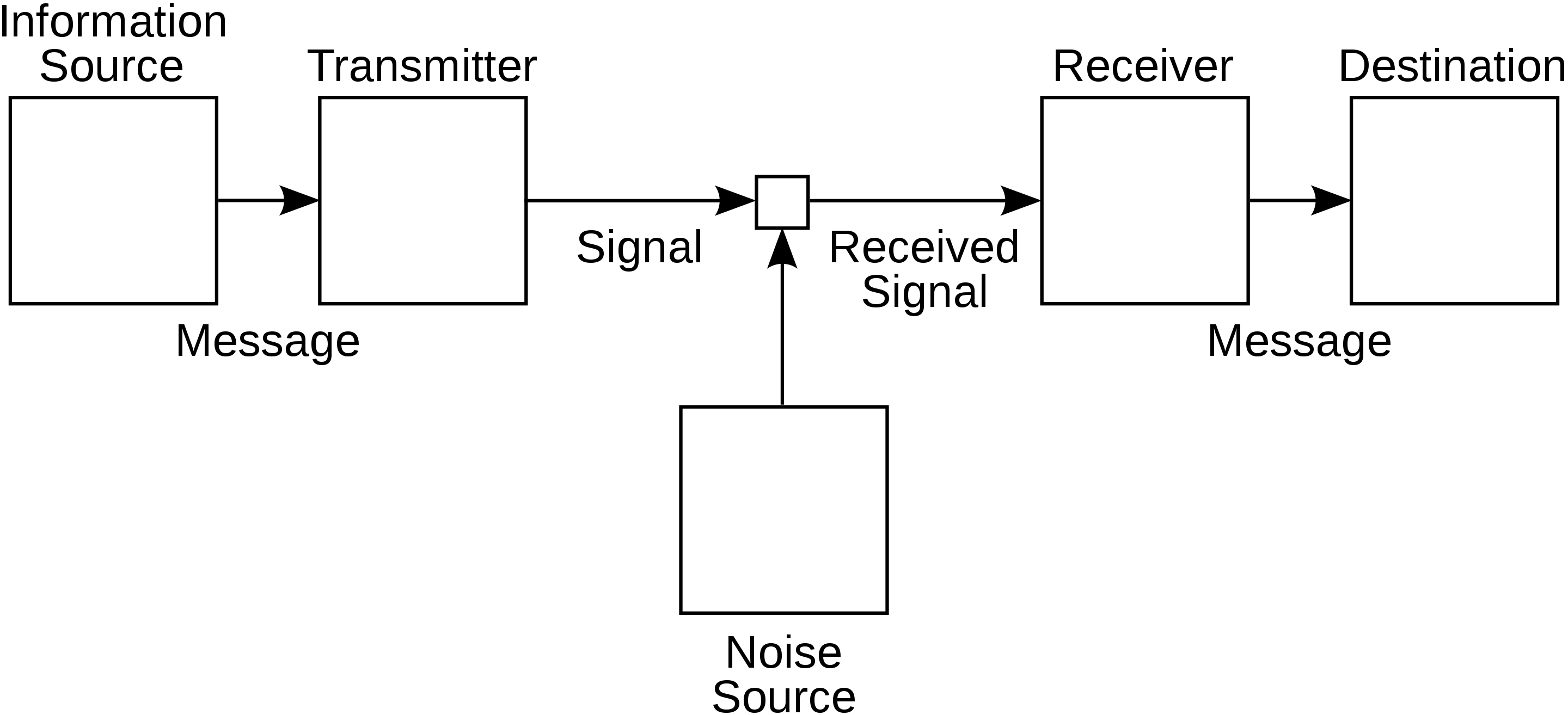
Figure 1: Image credit: Wikimedia Commons.
In Shannon’s model (our model of choice), the information source produces a message (in our case, a sequence of bits) that the transmitter turns into a signal (we will assume a modulator) and sends through the noisy channel. The receiver converts the signal back to a message (bit stream) and the bits reach their destination. Our modulator for the rest of this article will use binary phase shift keying (BPSK). This works by modulating the phase of the carrier, a single basis function that spans the signal space. For binary PSK, there are two possible phases, separated by \(\pi\) for each signal \(s_0(t)\) and \(s_1(t)\). We will choose:
\begin{align*} s_0(t) &= \sqrt{\frac{2E}{T}} \sin{\left(2\pi ft + \frac{\pi}{2} \right)}\\ s_1(t) &= \sqrt{\frac{2E}{T}} \sin{\left(2\pi ft - \frac{\pi}{2} \right)} \end{align*}where \(T\) is the time duration of the waveform, \(f\) is some multiple of \(1/T\), and \(E\) is the energy of each signal. We will now model the noise itself as additive white Gaussian noise (AWGN). Therefore, for a transmitted signal \(x(t)\), the received signal is modeled as \(y(t) = x(t) + n(t)\), where \(n(t)\) is a familiar Gaussian process, since we are modeling the sum of many random processes via the central limit theorem. Demodulating is interesting, since our we can ask our demodulator to make a decision. The sampled output by the decoder itself is a real number: \[\int_0^T x(t) \sqrt{\frac{2E}{T}}\sin{\left(2\pi ft + \frac{\pi}{2} \right)} dt\] This is unquantized. Our demodulator can either pass this “soft output” to the decoder itself (meaning the decoder has to be analog), or it can make a decision on how to map this real value to a discrete (in our case, binary) value, then pass the quantized “hard output” to the decoder. In our particular case, we will choose to map \(1\mapsto -1\) and \(0\mapsto +1\) in BPSK. This makes the XOR operation (addition modulo 2 in \(\mathbb{F}_2\)) equivalent to multiplication in the reals. Now, when the decoder receives a value of (for instance) \(-0.98\), it could make a decision to map this to \(-1\). This sets a threshold at 0: any value above zero maps to \(+1\) and any value below zero maps to \(-1\). This is a hard-decision decoder, and keeps implementation simple. However, for LDPC, we require a “soft” decoder, which will continue to use real values. This will be discussed further in the sections about SISO decoding.
Let us discuss in some more detail the errors that occur due to AWGN. In the case we are interested in, of BPSK over AWGN, we can use a simple and elegant model of our channel, the binary symmetric channel (BSC). Its model is simply a transition probability model:

Figure 2: Image credit: Wikimedia Commons.
where the “crossover” probability of a bit flip (an error) is \(p\) in both directions. In the next section, we discuss how to compute this probability, also called the bit error rate.
1.2. Signal to Noise Ratio and Bit Error Rate
Estimating the bit error rate (BER) via a Monte-Carlo simulation is quite intuitive, it is simply \[p\approx \frac{n_e}{N}\] where we transmit \(N\) bits and \(n_e\) of them are demodulated in error. The signal to noise ratio (SNR) is simply the ratio of the signal power to the noise power. The convention is to measure it in decibels, so our final expression is: \[\mathrm{SNR_{dB}} = 10\log_{10}{\left(\frac{P_{\text{signal}}}{P_{\text{noise}}} \right)}\] A trade-off is somewhat intuitive here: to decrease the BER, we can simply crank up the signal power, and hence increase the SNR. Using more power is not always a reasonable solution of course, so we press on. To formalize our notion of BER and SNR, we first show that the SNR in the continuous time domain and the discrete time domain is exactly the same. This allows us to restrict the rest of this article to the discrete time domain, which simplifies our analysis. For a signal in the continuous time domain with power \(P\), noise power spectral density \(\frac{N_0}2\), and bandwidth \(2W\), the SNR is simply \(\frac{P}{N_0W}\). For the discrete time domain, it is easier to consider energy per symbol \(E_s\) rather than channel power. If the symbol rate is \(T = \frac{1}{2W}\), we have that \(E_s = \frac{P}{2W}\). Computing the noise in discrete time is a bit involved, so we skip over it. The final result is that the noise energy is simply the variance \(\sigma^2=\frac{N_0}{2}\), the level of the noise PSD. Our expression for the SNR in the discrete time domain is therefore \(\frac{E_s}{\sigma^2}\). It is left to the reader to see that the SNR in both domains works out to the same expression. Henceforth, we simply work in discrete time.
For BPSK, \(E_s\) is rather easy to compute. It is simply given by: \[E_s = \frac{(-1)^2 + 1^2}{2} = 1\implies \text{SNR} = \frac{1}{\sigma^2}\] For BPSK over AWGN (effectively a BSC), the probability distribution of the noise is given by the Gaussian with variance \(\sigma^2\). If our transmitted symbol is \(t\) and our noise is \(n\), and we assume we have an equal probability of transmitting a \(+1\) or a \(-1\), our overall error rate is given by:
$$ \begin{align*}\text{BER} &= P(t = +1)\cdot P(n \leq -1) + P(t = -1)\cdot P(n \geq +1)\\[1em] &= \frac{1}{2}\cdot Q\left(\frac{1}{\sigma}\right) + \frac{1}{2}\cdot Q\left(\frac{1}{\sigma} \right) = Q\left(\frac{1}{\sigma} \right)\\[1em] &= Q\left(\sqrt{\text{SNR}} \right) \quad \text{where}\quad Q(x) := \frac{1}{2} \text{erfc}\left(\frac{x}{\sqrt{2}} \right) \end{align*} $$Although we’re glossing a bit over the math here, the takeaway is that for our model there is a simple relation between BER and SNR: \(\text{BER} = Q\left(\sqrt{\text{SNR}}\right)\).
1.2.1. Monte Carlo
To experimentally verify our math, let’s do a Monte Carlo simulation, and compare with the theoretical result:
import numpy as np
from math import erfc, sqrt


def theoretical_BER(sigma: float) -> float:
    def Q(x: float) -> float:
        return 0.5 * erfc(x / sqrt(2))

    return Q(1 / sigma)


def monte_carlo_BER(trials: int, sigma: float) -> float:
    signal = np.random.choice([-1, 1], size=(trials))
    noise = np.random.normal(0, sigma, trials)

    rcvd = signal + noise
    rcvd = [-1 if x < 0 else 1 for x in rcvd]

    errs = sum(1 for x, y in zip(signal, rcvd) if x != y)
    return errs / trials


sigma = 1
trials = 10**7
print(theoretical_BER(sigma), monte_carlo_BER(trials, sigma))
0.15865525393145705 0.1586437
1.2.2. Plotting BER and SNR
